

Creating an Arbitrary Waveform with the Rigol DG1022 Function/Arbitrary Waveform Generator
Using the Rigol DG1022 function generator to generate an arbitrary waveform is easy with just a few straightforward steps. You can use any program language (MATLAB is used here) and a USB flash drive along with the DG1022 to define and generate an arbitrary waveform. Included here are MATLAB scripts and example waveform files to make the job even easier.
Overview
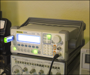
The Rigol DG1022 shown in Figure 1 is two-channel function generator with built-in waveforms and arbitrary waveform capabilities. An arbitrary waveform is a voltage-versus-time function that you define. To define an arbitrary waveform for the DG1022, choose a sequence of 4,096 values that range between 0 and 16,383, and the DG1022 will output those samples as a voltage waveform on one or both channels.
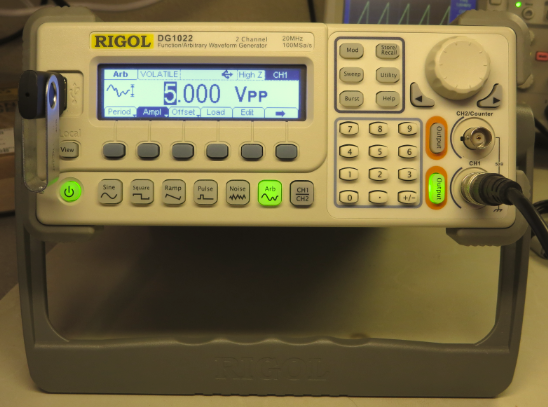
Figure 1. The Rigol DG1022 function generator has arbitrary waveform capabilities that are easy to use.
The DG1022 acts like a 14-bit digital-to-analog converter (DAC), “playing back” the sequence of values that you define. The instrument uses the amplitude (voltage limits) and period (sample rate) that you also define. Your complete waveform will be output repeatedly at the period you specify.
The steps described here to create and output an arbitrary waveform are:
- Conceptually define waveform.
- Create the binary waveform file (.rdf file) using MATLAB or any other software that saves an array of binary numbers to a file (e.g., C, Python, etc.).
- Load the file into the Rigol DG1022 using a USB flash drive.
- Define the amplitude (voltage limits of your waveform) and period (time duration of your waveform).
Other methods to create the waveform include using the DG1022 front panel to create a piecewise-linear function, using Rigol software, and using custom software that communicates with the function generator directly. I find creating my own binary file and transferring via a USB flash drive to be an easy method without the need for specialized software or numerous keystrokes.
The examples described here used a DG1022 with firmware version 00.02.00.06.00.02.07. Upon startup, the firmware version is shown on the screen in the location shown in Figure 2.
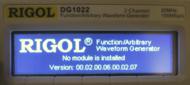
Figure 2. This article was written based on the firmware version shown on the screen in this figure.
Conceptually Defining the Waveform
To demonstrate the arbitrary waveform generator, I created two waveforms for the DG1022. The first waveform was a ramp waveform shown in Figure 3 that climbs linearly from 0 to 16,380 over 4,096 samples. The value increments by 4 for each sample increment. That is, sample 0 has value 0, sample 1 has value 4, sample 2 has value 8, …, and sample 4095 has value 13,380.
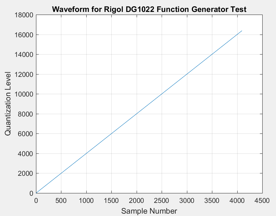
Figure 3. This ramp waveform was used as a simple test of the arbitrary waveform generator.
The second waveform demonstrates a more complicated shape. This waveform, nicknamed the “fancy” function, is shown in Figure 4.
- Samples 0 to 2,048 (0% to 50% of the waveform) are the first half-cycle of a sine wave.
- Samples 2,049 to 3,072 (50% to 75% of the waveform) have the value 8,192 (approximately half of 16,384).
- Samples 3,073 to 3,584 (75% to 87.5% of the waveform) have value 0.
- Samples 3,585 to 4,095 (87.5% to 100% of the waveform) have value 12,287 (approximately 75% of 16,384).
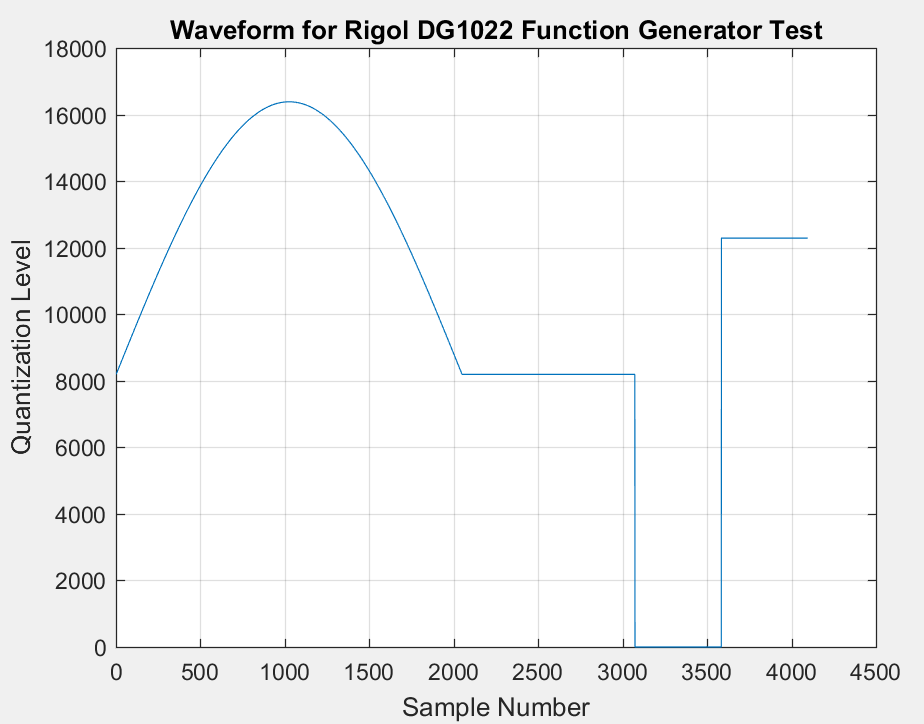
Figure 4. This “fancy” waveform was used to test the arbitrary waveform generator with a more complicate waveform.
This “fancy” waveform demonstrates that an arbitrarily defined waveform with curves and square features can be output from the DG1022.
Creating the Binary Waveform File
The DG1022 accepts a binary file to define a waveform. The binary waveform file has an .rdf extension and contains two bytes for each of the 4,096 samples. A brief description of the file format for the DG1000 series (and other Rigol function generators) is available on the Rigol website in the document named DG file format and arbitrary waveform examples.pdf (the version of the file used for this demo is linked here). This article provides additional details beyond the content of the Rigol document.
The value for each sample specifies a 14-bit quantization level. The range is:
- In decimal, 0 to 16,383 (0 to 214-1)
- In hexadecimal (hex), 0x0000 to 0x3FFF
The 14-bit value for each sample is stored in the 14 least-significant bits of each byte-pair in the file. The two most-significant bits are zeros. Files are in little-endian format, so that (for example) a value of 0x03AB would be written to the file in the order of AB 03.
The MATLAB command fwrite( fid, s, 'uint16', 'ieee-le' ) saves 16-bit data in the little-endian format. The MATLAB .m script linked here creates a binary waveform file for the ramp waveform that can be loaded into the DG1022:
This is the .rdf waveform file that the MATLAB script creates:
When Ramp.pdf is opened in Notepad++, and viewed with the hex editor (Plugins→HEX-Editor), the RDF file looks like the screen capture in Figure 5.
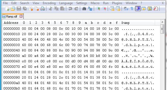
Figure 5. The hex editor in Notepad++ shows the Ramp.rdf file containing the ramp waveform data in little-endian format.
The file contents show that the first sample (value 0x0000 = 0) is stored as 00 00 in the first two bytes, and the second sample (value 0x0004 = 4) is stored as 04 00 in the second four bytes.
To create the “fancy” function, use this MATLAB script:
This is the .rdf waveform file that the MATLAB script creates:
Both of the binary waveform (.rdf) files above can be loaded directly into the DG1022.
Loading the File into the DG1022
To load a binary waveform file into the DG1022, copy the file from the PC to the root folder of a USB flash drive formatted in FAT32 or FAT format (FAT16 is displayed as “FAT” in the format dialog box in Windows 10). I tried using a USB flash drive formatted for NTFS, and the DG1022 could not read files from it. Both FAT32 and FAT worked for me.
Select either channel 1 or channel 2 with the Ch1/Ch2 button on the DG1022 to load the waveform into the corresponding channel. Insert the USB stick with the binary waveform file (.rdf) into the USB port on the DG1022 front panel. Press the Arb button, and then select the Load soft key (Arb→Load). The “UDisk” label should show on the display when a USB flash drive is present. Press the Disk soft key to highlight the “UDisk” label, and a list of files on the USB flash drive should appear.
Roll the front-panel knob to select the desired binary waveform (.rdf) file, and press the Recall soft key. The waveform should now be loaded into the DG1022. Turning on the output (channel 1 or channel 2 as originally selected) will produce the waveform at the corresponding output connector of the function generator.
Defining the Amplitude and Period of the Waveform
The mapping of quantization levels (0 to 16,383) to volts is defined using the amplitude and offset settings (see Figure 6). Amplitude is set using Arb→Ampl. The amplitude setting controls the voltage difference between the 16,383 quantization level and the 0 quantization level. The voltage offset is set using Arb→Offset. For example, if the amplitude is set to 5 V and the offset is set to 0 V, then the 0 quantization level will output -2.5 V, and the 16,383 quantization level will output +2.5 V. If the amplitude is set to 5 V and the offset is set to 2 V, then the 0 quantization level will output -0.5 V, and the 16,383 quantization level will output +4.5 V.
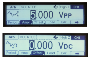
Figure 6. The amplitude setting (top) and offset setting (bottom) control the voltage scaling of the arbitrary waveform.
Configure the time scale of the entire waveform using Arb→Period (see Figure 7). (Press the Arb→Freq button twice to switch from Freq to Period.) The period sets the time duration over which the entire waveform is output and then repeats.
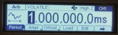
Figure 7. The period setting controls the time scaling of the arbitrary waveform.
The period setting essentially controls the output sample rate for the arbitrary waveform.
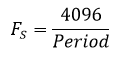
For example, when the period is set to 1 ms, the sample rate FS is 4,096 Samples / 0.001 seconds = 4.096 MS/s.
Pressing the Period button until Freq appears allows control using the unit of sequences per second. The sample rate is then calculated using
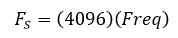
For example, if the frequency is set to 1 KHz, then the sample rate FS is (4,096 Samples)(1000 Hz) = 4,096 MS/s.
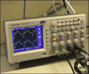
Measured Waveforms
After loading the Ramp.rdf into the DG1022, I set the amplitude to 5 V peak-to-peak and the period to 1 ms. When the output was enabled and viewed on an oscilloscope, the binary waveform file Ramp.rdf produced the waveform shown in the oscilloscope screen capture in Figure 8. The waveform looks as expected, with a 5 V peak-to-peak voltage span and a ramp function that repeats every 1 ms.
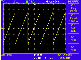
Figure 8. The measured ramp waveform matches the defined ramp waveform.
Next, I loaded the FancyFunction.rdf into the DG1022 using the same amplitude and period settings (5 V peak-to-peak and 1 ms, respectively). The waveform also looked exactly as expected, and it was amusing seeing the measured waveform in Figure 9 on an oscilloscope.
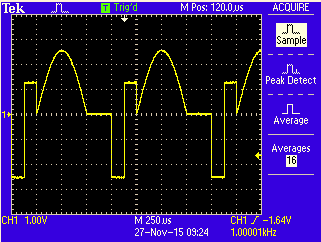
Figure 9. The measured “fancy” waveform shows that complicated shapes can be created.
Summary of Key Points & Tips
Here are keys to getting an arbitrary waveform up and running:
- The waveform file that you create should contain 4,096 values that will be converted to a voltage waveform and “played back” by the DG1022 over and over again.
- Each value can range from 0 to 16,383 (0 to 214-1) (0x0000 to 0x3FFF in hexadecimal).
- Each value should be stored in a binary file as an unsigned, 16-bit binary word in little-endian format.
- The USB flash drive used to transfer the file must be formatted using FAT32 or FAT (not NTFS).
- If fewer than 4,096 values (say, N values) are contained in the binary file and loaded into the function generator, then only the first N values present in the function generator are changed, and the remaining values present in the function generator remain unchanged.
- Use the amplitude and period settings to configure the voltage span and rate of your waveform.
Creating arbitrary waveforms with the Rigol DG1022 is that easy, and this capability to produce a wide variety of waveform shapes is a great addition to an engineer’s toolbox.
